AAWSAP DIRD, Quantum Tomography of Negative Energy States in the Vacuum, January 2011

Text

This text came with the file. It may have mistakes. When the text and the image disagree, the image is right.

UNCLASSIFIED//PO" OPPICIJ!tt l:191! OHL'f
detector
I vacuum
'Y.
detector
I b
signal
a
a'
local
oscillator
(aLO)
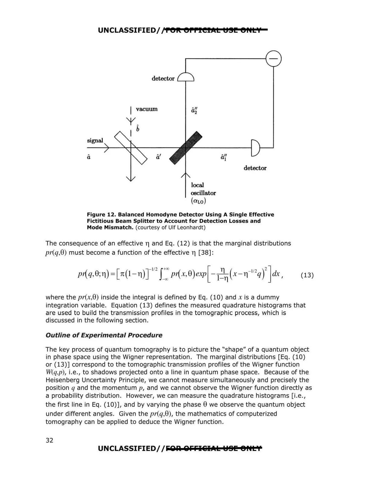
Figure 12. Balanced Homodyne Detector Using A Single Effective
Fictitious Beam Splitter to Account for Detection Losses and
Mode Mismatch. (courtesy of Ulf Leonhardt)
The consequence of an effective 17 and Eq. {12) is that the marginal distributions
pr(q,0) must become a function of the effective 17 [38]:
where the pr(x,0) inside the integral is defined by Eq. (10) and x is a dummy
integration variable. Equation (13) defines the measured quadrature histograms that
are used to build the transmission profiles in the tomographic process, which is
discussed in the following section.
Outline of Experimental Procedure
The key process of quantum tomography is to picture the "shape" of a quantum object
in phase space using the Wigner representation. The marginal distributions [Eq. (10)
or (13)] correspond to the tomographic transmission profiles of the Wigner function
W(q,p), i.e., to shadows projected onto a line in quantum phase space. Because of the
Heisenberg Uncertainty Principle, we cannot measure simultaneously and precisely the
position q and the momentum p, and we cannot observe the Wigner function directly as
a probability distribution. However, we can measure the quadrature histograms [i.e.,
the first line in Eq. (10)], and by varying the phase 0 we observe the quantum object
under different angles. Given the pr(q,0), the mathematics of computerized
tomography can be applied to deduce the Wigner function.
UNCLASSIFIED//FOA OFFI&:iI.t.l:: Y81!! 8HLY
32