AAWSAP DIRD, An Introduction to the Statistical Drake Equation, March 2010

Text

This text came with the file. It may have mistakes. When the text and the image disagree, the image is right.

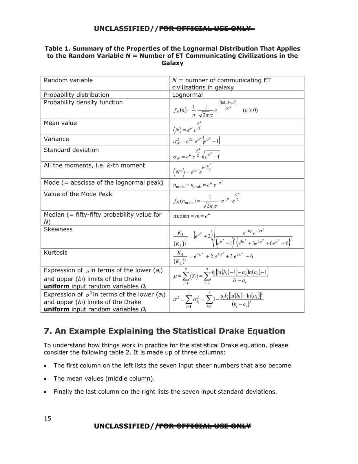
UNCLASSIFIED/ /FOR OFFIEiIAk Wlii QPU,¥
Table 1. Summary of the Properties of the Lognormal Distribution That Applies
to the Random Variable N = Number of ET Communicating Civilizations in the
Galaxy
Random variable
N = number of communicating ET
civilizations in galaxy
Probability distribution
Loqnormal
Probability density function
(1n(11h,J'
1
1
-~ (n ;::-: 0)
n
27!<:T
JN (n)= - · &
e
a'
Mean value
-
(N )= eµe 2
Variance
a1 = e2µ ea' (ea' - I)
a'
a N = eµ e 2 .Jea2 - 1
Standard deviation
All the moments, i.e. k-th moment
2 a'
k ·­2
(N k)= ekµ e
_
_ ~I
- a-2
Mode (= abscissa of the log normal peak)
n nnde = npeak - e e
a'
f (
)
Value of the Mode Peak
1
-p 2
N n lTl)dc = &
·e
·e
2,r (l
Median (= fifty-fifty probability value for
rred ian =m =e"
N)
Skewness
K
( ,
)
e-6pe-3a'
_
3_ = ea + 2
(K4)¾
.,
lne3a2 + 3e2a' +6ea' +61
k' ­
K
,,
.,
.,
"}
Kurtosis
_
4_ = e4a- + 2 e3a- + 3 e-u- - 6
(K2)2
Expression of 1-1 in terms of the lower (a;)
µ = ± (Y;) =± b;[in(b;) - 1]- a;[in(a;)-1]
and upper (b;) limits of the Drake
i=I
i= I
b; - a;
uniform input random variables 0 ;
Expression of <:T 2 in terms of the lower (a;)
7
7
a;b;[ln (b; )- in(a;)f
a 2 =La~ = L l­
and upper (b;) limits of the Drake
(b;-a}
i= I
i=I
uniform input random variables 0 ;
7. An Example Explaining the Statistical Drake Equation
To understand how things work in practice for the statistical Drake equation, please
consider the following table 2. It is made up of three columns:
•
The first column on the left lists the seven input sheer numbers that also become
•
The mean values (middle column).
•
Finally the last column on the right lists the seven input standard deviations.
UNCLASSIFIED/1re1t OFFl@IAL WSE 9Nk¥
15