AAWSAP DIRD, An Introduction to the Statistical Drake Equation, March 2010

Text

This text came with the file. It may have mistakes. When the text and the image disagree, the image is right.

UNCLASSIFIED/ /FOR OFFI&IAk Wlii QPU,¥
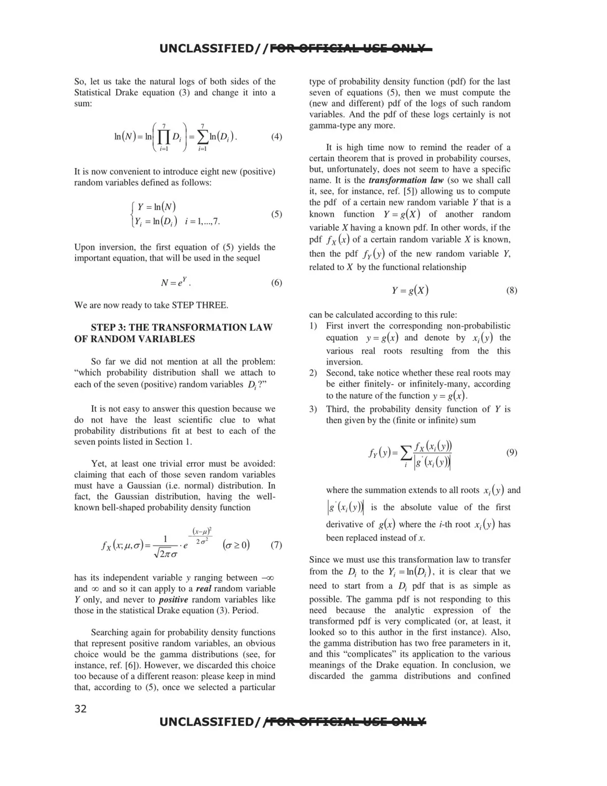
So, let us take the natural logs of both sides of the
Statistical Drake equation (3) and change it into a
sum:
It is now convenient to introduce eight new (positive)
random variables defined as follows:
Y=ln(N)
{
(5)
Y;=ln(D;) i=l,...,7.
Upon inversion, the first equation of (5) yields the
important equation, that will be used in the sequel
(6)
We are now ready to take STEP THREE.
STEP 3: THE TRANSFORMATION LAW
OF RANDOM VARIABLES
So far we did not mention at all the problem:
"which probability disttibution shall we attach to
each of the seven (positive) random variables D; ?"
It is not easy to answer this question because we
do not have the least scientific clue to what
probability distributions fit at best to each of the
seven points listed in Section 1.
Yet, at least one trivial error must be avoided:
claiming that each of those seven random variables
must have a Gaussian (i.e. normal) distribution. In
fact, the Gaussian distribution, having the well­
known bell-shaped probability density function
(a ;,: o)
(7)
has its independent variable y ranging between --oo
and oo and so it can apply to a real random variable
Y only, and never to positive random variables like
those in the statistical Drake equation (3). Period.
Searching again for probability density functions
that represent positive random variables, an obvious
choice would be the gamma distributions (see, for
instance, ref. [6]). However, we discarded this choice
too because of a different reason: please keep in mind
that, according to (5), once we selected a particular
type of probability density function (pdt) for the last
seven of equations (5), then we must compute the
(new and different) pdf of the logs of such random
variables. And the pdf of these logs certainly is not
gamma-type any more.
It is high time now to remind the reader of a
certain theorem that is proved in probability courses,
but, unfortunately, does not seem to have a specific
name. It is the transformation law (so we shall call
it, see, for instance, ref. [5]) allowing us to compute
the pdf of a certain new random variable Y that is a
known
function Y=g(X) of another random
variable X having a known pdf. In other words, if the
pdf fx (x) of a certain random variable X is known,
then the pdf fr(Y) of the new random variable Y,
related to X by the functional relationship
y = g(X)
(8)
can be calculated according to this rule:
1)
First invert the corresponding non-probabilistic
equation y =g(x) and denote by
X; (y) the
various real roots resulting from the this
inversion.
2)
Second, take notice whether these real roots may
be either finitely- or infinitely-many, according
to the nature of the function y = g(x).
3) Third, the probability density function of Y is
then given by the (finite or infinite) sum
(9)
where the summation extends to all roots x;(Y) and
lg' (x; (y)~ is the absolute value of the first
derivative of g(x) where the i-th root x;(Y) has
been replaced instead of x.
Since we must use this transformation law to transfer
from the D; to the Y; =ln(D;), it is clear that we
need to start from a D; pdf that is as simple as
possible. The gamma pdf is not responding to this
need
because the analytic expression of the
transformed pdf is very complicated (or, at least, it
looked so to this author in the first instance). Also,
the gamma distribution has two free parameters in it,
and this "complicates" its application to the various
meanings of the Drake equation. Tn conclusion, we
discarded the gamma distributions and confined
UNCLASSIFIED/ /FOil OFFI@IAb W&i! QNI.¥
32