AAWSAP DIRD, An Introduction to the Statistical Drake Equation, March 2010

Text

This text came with the file. It may have mistakes. When the text and the image disagree, the image is right.

UNCLASSIFIED/ /fOR OFFI&IAk Wlii QPU,¥
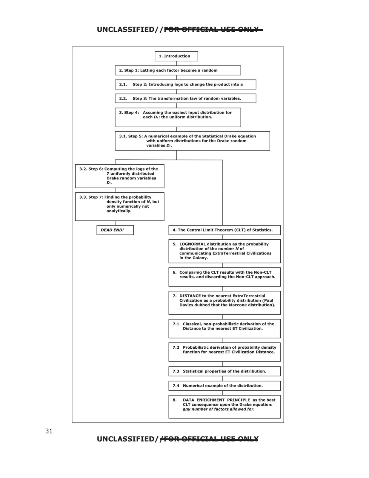
I 1. Introduction I
I
2. Step 1: Letting each factor become a random
I
2.1.
Step 2: Introducing logs to change the product into a
I
I
2.2.
Step 3: The transformation law of random variables.
I
I
3. Step 4: Assuming the easiest input distribution for
each D1: the uniform distribution.
I
3.1. Step 5: A numerical example of the Statistical Drake equation
with uniform distributions for the Drake random
variables 0 ;.
I
3.2. Step 6: Computing the logs of the
7 uniformly distributed
Drake random variables
O; .
I
3.3. Step 7: Finding the probability
I
density function of N, but
only numerically not
analytically.
I
DEAD END! I
4. The Central Limit Theorem (CLT) of Statistics.
I
s. LOGNORMAL distribution as the probability
distribution of the number N of
communicating ExtraTerrestrial Civilizations
in the Galaxy.
I
6. Comparing the CLT results with the Non-CLT
results, and discarding the Non-CLT approach.
7. DISTANCE to the nearest ExtraTerrestriai
Civilization as a probability distribution ( Paul
Davies dubbed that the Maccone distribution).
I
7.1 Classical, non-probabilistic derivation of the
Distance to the nearest ET Civilization.
7.2 Probabilistic derivation of probability density
function for nearest ET Civilization Distance.
7.3 Statistical properties of the distribution.
7.4 Numerical example of the distribution.
I
8.
DATA ENRICHMENT PRINCIPLE as the best
CLT consequence upon the Drake equation:
;mx number of factors allowed for.
UNCLASSIFIED/ ;'FQA QFFICilPL. PP&i ODI! Y
31