AAWSAP DIRD, An Introduction to the Statistical Drake Equation, March 2010

Text

This text came with the file. It may have mistakes. When the text and the image disagree, the image is right.

UNCLASSIFIED/ /FOR OFFI&IAk Wlii QPU,¥
In other words, there is a factor of ✓3 =1.732
included in the two equations (17) that is not obvious
at all to human intuition, and must indeed be taken
into account.
The application of this result to the Statistical Drake
equation is discussed in the next section.
3.1 STEP 5: A NUMERICAL EXAMPLE
OF THE STATISTICAL DRAKE
EQUATION WITH UNIFORM
DISTRIBUTIO S FOR THE DRAKE
RANDOM VARIABLES D;
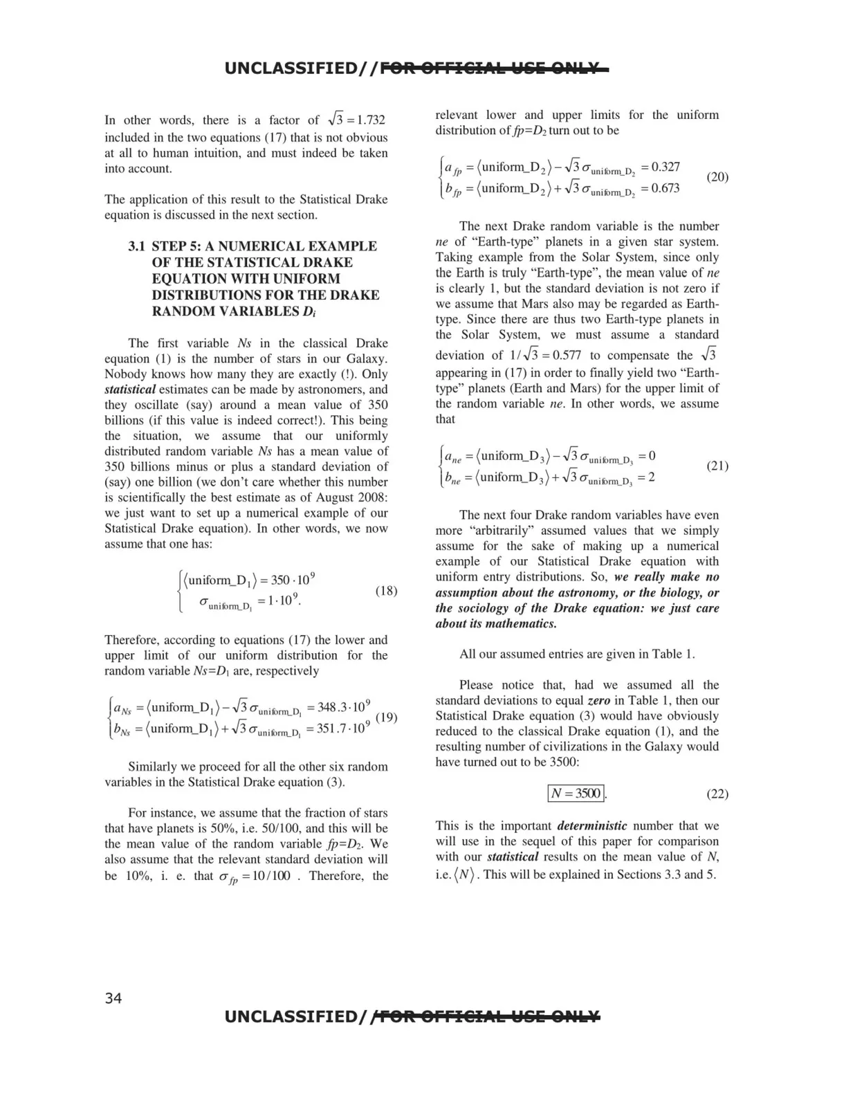
The first variable Ns in the classical Drake
equation (1) is the number of stars in our Galaxy.
Nobody knows how many they are exactly (!). Only
statistical estimates can be made by astronomers, and
they oscillate (say) around a mean value of 350
billions (if this value is indeed correct!). This being
the situation,
we
assume that our uniformly
distributed random variable Ns has a mean value of
350 billions minus or plus a standard deviation of
(say) one billion (we don't care whether this number
is scientifically the best estimate as of August 2008:
we just want to set up a numerical example of our
Statistical Drake equation). ln other words, we now
assume that one has:
(uniform_D 1) =350 ~109
{
(18)
a unilomLD, =l • 10 •
Therefore, according to equations (17) the lower and
upper limit of our uniform distribution for the
random variable Ns=D1 are, respectively
aNs = 1 uniform_D 1 ) - ✓3auni "'" rm O = 348.3-109
{
\
.
,v
-
I
9 ( ( 9)
bNs =(umform_D 1) + ,fj aunii:>rTTLD, =351.7 -10
Similarly we proceed for all the other six random
variables in the Statistical Drake equation (3).
For instance, we assume that the fraction of stars
that have planets is 50%, i.e. 50/100, and this will be
the mean value of the random variable fp=D2. We
also assume that the relevant standard deviation will
be 10%, i. e. that a fr =10 /100 . Therefore, the
relevant lower and upper limits for the uniform
distribution offp=D2 tum out to be
a fp : ( un~orm_D2 )- ,fj a unitbrnLD2 : 0.327
(20)
{
b.fp - ( uniform_D 2 ) + ,fj a unitomLD2 - 0.673
The next Drake random variable is the number
ne of "Earth-type" planets in a given star system.
Taking example from the Solar System, since only
the Earth is truly "Earth-type", the mean value of ne
is clearly I, but the standard deviation is not zero if
we assume that Mars also may be regarded as Earth­
type. Since there are thus two Earth-type planets in
the Solar System, we must assume a standard
deviation of 1 / ,fj =0.577 to compensate the ,fj
appearing in (17) in order to finally yield two "Earth­
type" planets (Earth and Mars) for the upper limit of
the random variable ne. In other words, we assume
that
The next four Drake random variables have even
more "arbitrarily" assumed values that we simply
assume for the sake of making up a numerical
example of our Statistical Drake equation with
uniform entry distributions. So, we really make no
assumption about the astronomy, or the biology, or
the sociology of the Drake equation: we just care
about its mathematics.
All our assumed entries are given in Table l.
Please notice that, had we assumed all the
standard deviations to equal zero in Table I, then our
Statistical Drake equation (3) would have obviously
reduced to the classical Drake equation (1), and the
resulting number of civilizations in the Galaxy would
have turned out to be 3500:
IN =3500 1.
(22)
This is the important deterministic number that we
will use in the sequel of this paper for comparison
with our statistical results on the mean value of N,
i.e. (N). This will be explained in Sections 3.3 and 5.
UNCLASSIFIED// POil OFFI@IAb W&i 01'11.¥
34