AAWSAP DIRD, An Introduction to the Statistical Drake Equation, March 2010

Text

This text came with the file. It may have mistakes. When the text and the image disagree, the image is right.

=
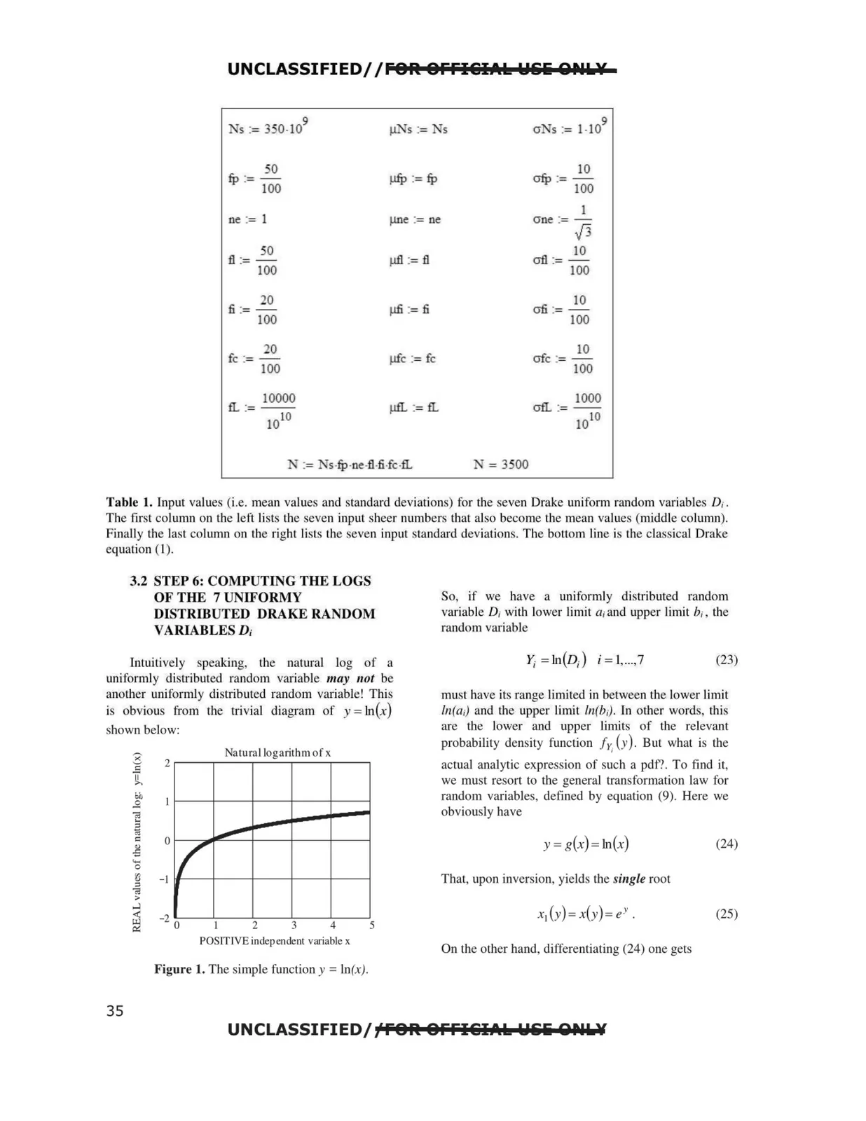
UNCLASSIFIED/ /FOR OFFIEil.t.k W&i Q~lls¥
1s := 3 · o-109
s := -s
cr s := 1-109
·o
10
µfp := fp
fp := 100
crfp := 100
1
ne := 1
µne := ne
crne := ­,/3
fl :=~
µfl := fl
crt1 = ~
100
100
fi := 20
µfi := fi
crfi := ~
100
100
fc := 20
-100
µfc := fc
10
crfc := -100
10000
fl. :=--
µfl. := fl.
1000
crfl. := --
1010
101 0
s-fp -ne­fl-fi.fc .fl.
- = 3500
Table 1. Input values (i.e. mean values and standard deviations) for the seven Drake uniform random variables D;.
The fi rst column on the left lists the seven input sheer numbers that also become the mean values (middle column).
Finally the last column on the right lists the seven input standard deviations. The bottom line is the classical Drake
equation (1).
3.2 STEP 6: COMPUTING THE LOGS
OF THE 7 UNIFORMY
DISTRIBUTED DRAKE RANDOM
VARIABLES D;
Intuiti vely speakiJ1g, the natural log of a
unifonnly disuibuted random variable may not be
another uniformly distributed random variable! This
is obvious from the tri vial diagram of y =ln (x)
shown below:
Natural logarithm of x
-
_,,,,,,,,_,,. ~
r
2
3
4
5
POSITIVE independent variable x
Figure 1. The simple function y = ln(x).
So, if we have a uniformly distributed random
variable D; with lower limit a;and upper limit b;, the
random variable
Y; =ln(D;) i = l,...,7
(23)
must have its range limited in between the lower limit
l11(a;) and the upper limi t ln(b,). In other words, this
are the lower and upper limits of the relevant
probability density function fr;(y). But what is the
actual analytic expression of such a pdf/. To find it,
we must resort to the general transformation law for
random variables, defined by equation (9). Here we
obviously have
y =g(x) =ln(x)
(24)
That, upon inversion, yields the single root
(25)
On the other hand, differentiating (24) one gets
UNCLASSIFIED//FOR OFFIEil.t.k W&i QNls¥
35