Department of the Air Force Report, 1996

Text

This text came with the file. It may have mistakes. When the text and the image disagree, the image is right.

the differences in calculated Mode-5 risks for the different values of B would surely
have been less.
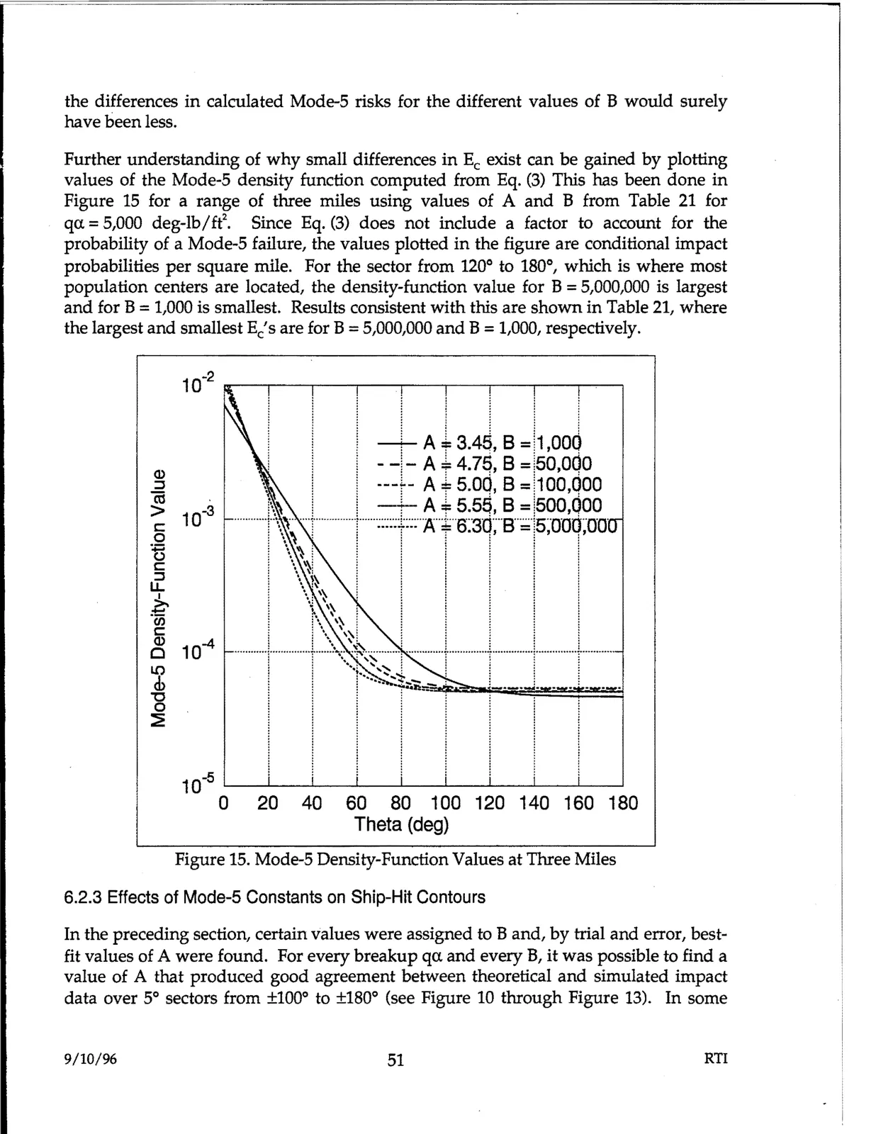
Further understanding of why small differences in Ee exist can be gained by plotting
values of the Mode-5 density function computed from Eq. (3) This has been done in
Figure 15 for a range of three miles using values of A and B from Table 21 for
qa. =5,000 deg-lb/ft2.
Since Eq. (3) does not include a factor to account for the
probability of a Mode-5 failure, the values plotted in the figure are conditional impact
probabilities per square mile. For the sector from 120° to 180°, which is where most
population centers are located, the density-function value for B =5,000,000 is largest
and for B =1,000 is smallest. Results consistent with this are shown in Table 21, where
the largest and smallest Ec's are for B =5,000,000 and B =1,000, respectively.
~ ~ 00
00 1001~1~100100
Theta (deg)
Figure 15. Mode-5 Density-Function Values at Three Miles
6.2.3 Effects of Mode-5 Constants on Ship-Hit Contours
In the preceding section, certain values were assigned to Band, by trial and error, best-
fit values of A were found. For every breakup qa. and every B, it was possible to find a
value of A that produced good agreement between theoretical and simulated impact
data over 5° sectors from ±100° to ±180° (see Figure 10 through Figure 13). In some
9/10/96
51
RTI