AAWSAP DIRD, An Introduction to the Statistical Drake Equation, March 2010

Text

This text came with the file. It may have mistakes. When the text and the image disagree, the image is right.

•
•
UNCLASSIFIED/ /fOR OFFI&IAk Wlii QPU,¥
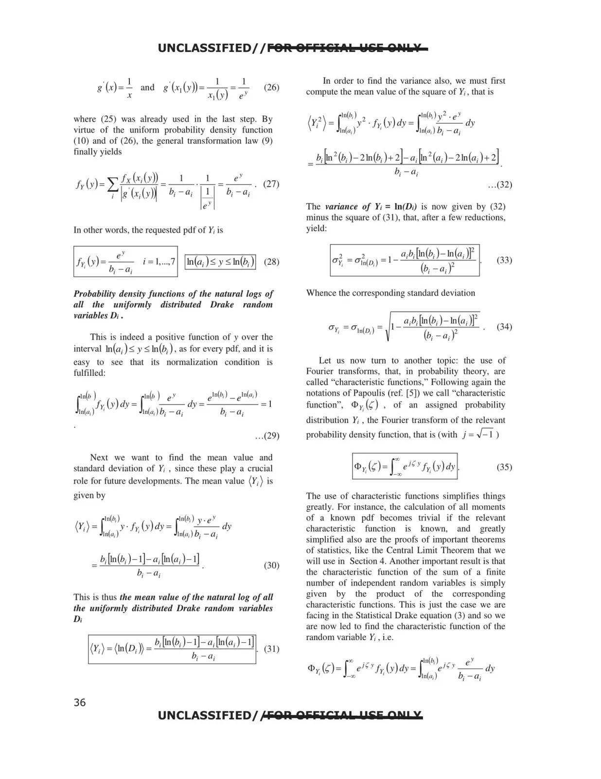
where (25) was already used in the last step. By
virtue of the uniform probability density function
(I 0) and of (26), the general transformation law (9)
finally yields
1n other words, the requested pdf of Y; is
eY
,--,---,,-----,-.,..,
fr,(y) =--
i = l, ...,7 lm(a;) :,;y:,;in(b;)I (28)
b; - a;
Probability density functions of the natural logs of
all the
uniformly distributed Drake
random
variables D; .
This is indeed a positive function of y over the
interval !n(a;):,; y:,; ln(b;) , as for every pdf, and it is
easy to see that its normalization condition is
fulfilled:
... (29)
Next we want to find the mean value and
standard deviation of Y; , since these play a crucial
role for future developments. The mean value (Y;) is
given by
!n(b;)
( )
s.•n(b;) y,eY
(Y.) = J.
Y· fr y dy =
-- dy
1
Jn(a,)
'
!n(a,)b; -a;
b; [in(b; )-1]- a,-[in(a; )-1]
= --'-''----''--'--'--=--'-"-"--'-'---=
(30)
This is thus the mean value of the natural log of all
the uniformly distributed Drake random variables
D;
In order to find the variance also, we must first
compute the mean value of the square of Y;, that is
( 2)
J.in(b.) 2
{ .)
J.!n(/J.) y2 •e Y
Y; =
y ·fry dy=
--dy
h1(<1;)
'
!n(a;) b; - Cl;
= b; ~
2(b; )- 21n(b; )+ 2]- a; [ln 2 (a; )- 2ln(a; )+ 2)
b; - a;
... (32)
The variance of Y; = ln(D;) is now given by (32)
minus the square of (31), that, after a few reductions,
yield:
2
2
a.b.[ln(b.)- ln(a .)]2
a - a
_ 1_ , ,
,
,
(33)
r, -
In(o,) -
(b; _ a;)2
Whence the corresponding standard deviation
1 _ a;b; [in(b;)- in(a;)]2
(34)
(b; - a;)2
Let us now turn to another topic: the use of
Fourier transforms, that, in probability theory, are
called "characteristic functions," Following again the
notations of Papoulis (ref. [5]) we call "characteristic
function", <Dy, (s) , of an assigned probability
distribution Y; , the Fourier transform of the relevant
probability density function, that is (with j = ~)
The use of characteristic functions simplifies things
greatly. For instance, the calculation of all moments
of a known pdf becomes trivial if the relevant
characteristic
function
is
known,
and
greatly
simplified also are the proofs of important theorems
of statistics, like the Central Limit Theorem that we
will use in Section 4. Another important result is that
the characteristic function of the sum of a finite
number of independent random variables is simply
given
by
the
product of the
corresponding
characteristic functions. This is just the case we are
facing in the Statistical Drake equation (3) and so we
are now led to find the characteristic function of the
random variable Y; , i.e.
UNCLASSIFIED/,'FOA OFlilCI0 I. P !SE ON! X
36