AAWSAP DIRD, An Introduction to the Statistical Drake Equation, March 2010

Text

This text came with the file. It may have mistakes. When the text and the image disagree, the image is right.

UNCLASSIFIED/ /fOR OFFI&IAk Wlii QPU,¥
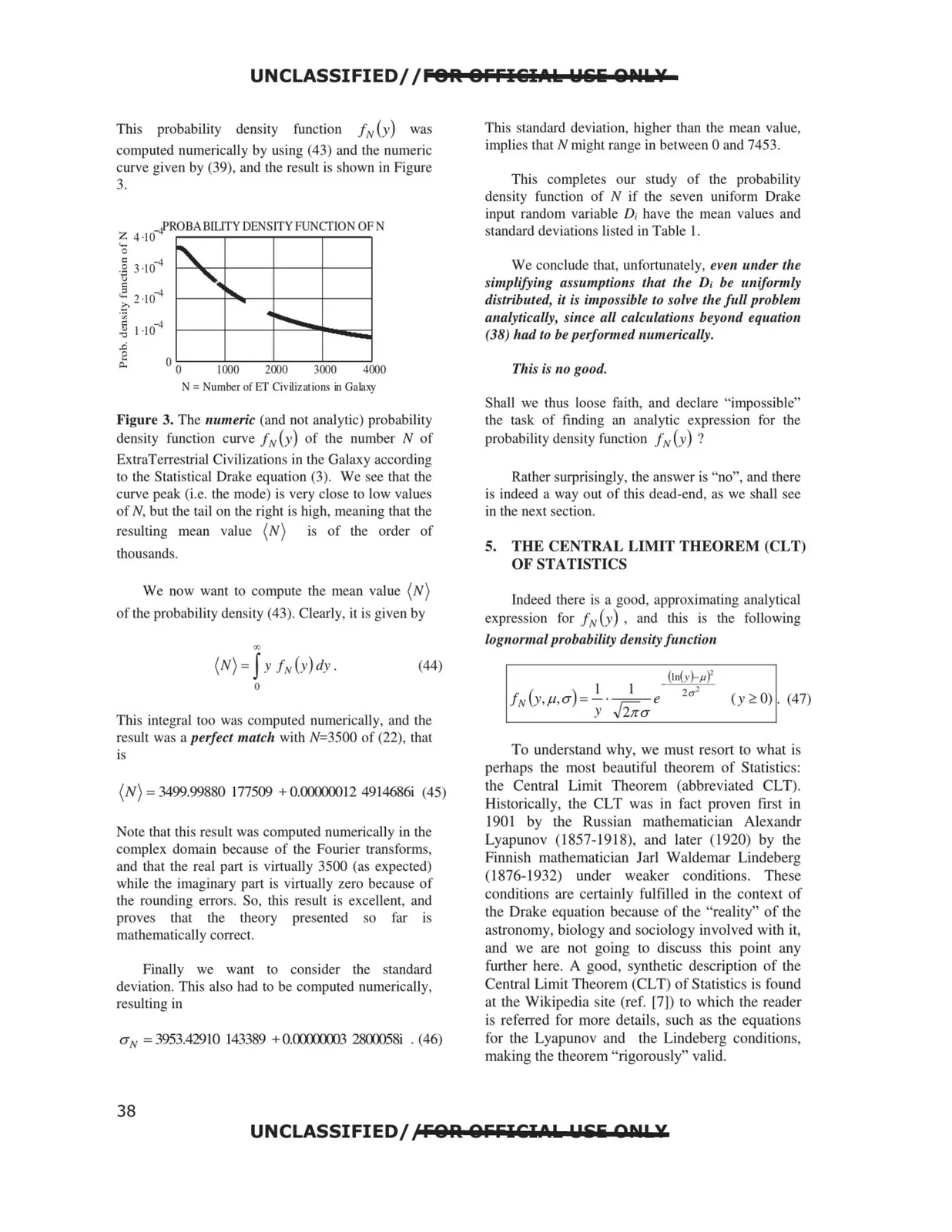
This
probability density
function
f N (y)
was
computed numerically by using (43) and the numeric
curve given by (39), and the result is shown in Figure
3.
Z 4 · l 0-4PROBA BILITY DENSITY FUNCTIO OF N
.....
0 .g 3·10-4
{)
C:
..: 2·10-4
·i
~ 1 ·10-4
1000
2000
3000
4000
N = umber of ET Civilizations in Galaxy
Figure 3. The numeric (and not analytic) probability
density function curve f N (y) of the number N of
ExtraTerrestrial Civilizations in the Galaxy according
to the Statistical Drake equation (3). We see that the
curve peak (i.e. the mode) is very close to low values
of N, but the tail on the right is high, meaning that the
resulting mean value (N)
is of the order of
thousands.
We now want to compute the mean value (N)
of the probability density (43). Clearly, it is given by
(N) =f
00
y J,v(y)dy.
(44)
0
This integral too was computed numerically, and the
result was a perfect match with N=3500 of (22), that
is
(N) = 3499.99880 177509 + 0.OOCXX:XH2 4914686i (45)
Note that this result was computed numerically in the
complex domain because of the Fourier transforms,
and that the real part is virtually 3500 (as expected)
while the imaginary part is virtually zero because of
the rounding errors. So, this result is excellent, and
proves
that
the
theory
presented
so
far
is
mathematically correct.
Finally we want to consider the standard
deviation. This also had to be computed numerically,
resulting in
uN =3953.42910 143389 +o.cx:x:x:x:x:m 28CXXJ58i . (46)
This standard deviation, higher than the mean value,
implies that N might range in between 0 and 7453.
This completes our study of the probability
density function of N if the seven uniform Drake
input random variable D; have the mean values and
standard deviations listed in Table I .
We conclude that, unfortunately, even under the
simplifying assumptions that the D; be 11nifor111ly
distributed, it is impossible to solve the full problem
a11alytically, since all calculations beyond equation
(38) had to be performed numerically.
This is no good.
Shall we thus loose faith, and declare "impossible"
the task of finding an analytic expression for the
probability density function f N (y) ?
Rather surprisingly, the answer is "no", and there
is indeed a way out of this dead-end, as we shall see
in the next section.
5.
THE CENTRAL LIMIT THEOREM (CLT)
OF STATISTICS
Indeed there is a good, approximating analytical
expression for ftv (y) , and this is the following
lognormal probability density Junction
To understand why, we must resort to what is
perhaps the most beautiful theorem of Statistics:
the Central Limit Theorem (abbreviated CLT).
Historically, the CLT was in fact proven first in
190 I by the Russian mathematician Alexandr
Lyapunov (1857-1918), and later (1920) by the
Finnish mathematician Jar! Waldemar Lindeberg
(1876-1932) under weaker conditions. These
conditions are certainly fulfilled in the context of
the Drake equation because of the "reality" of the
astronomy, biology and sociology involved with it,
and we are not going to discuss this point any
further here. A good, synthetic description of the
Central Limit Theorem (CLT) of Statistics is found
at the Wikipedia site (ref. (7)) to which the reader
is refetTed for more details, such as the equations
for the Lyapunov and the Lindeberg conditions,
making the theorem "rigorously" valid.
UNCLASSIFIED/ J'FQA QFFICiIPL. !Iii 011! X
38