AAWSAP DIRD, An Introduction to the Statistical Drake Equation, March 2010

Text

This text came with the file. It may have mistakes. When the text and the image disagree, the image is right.

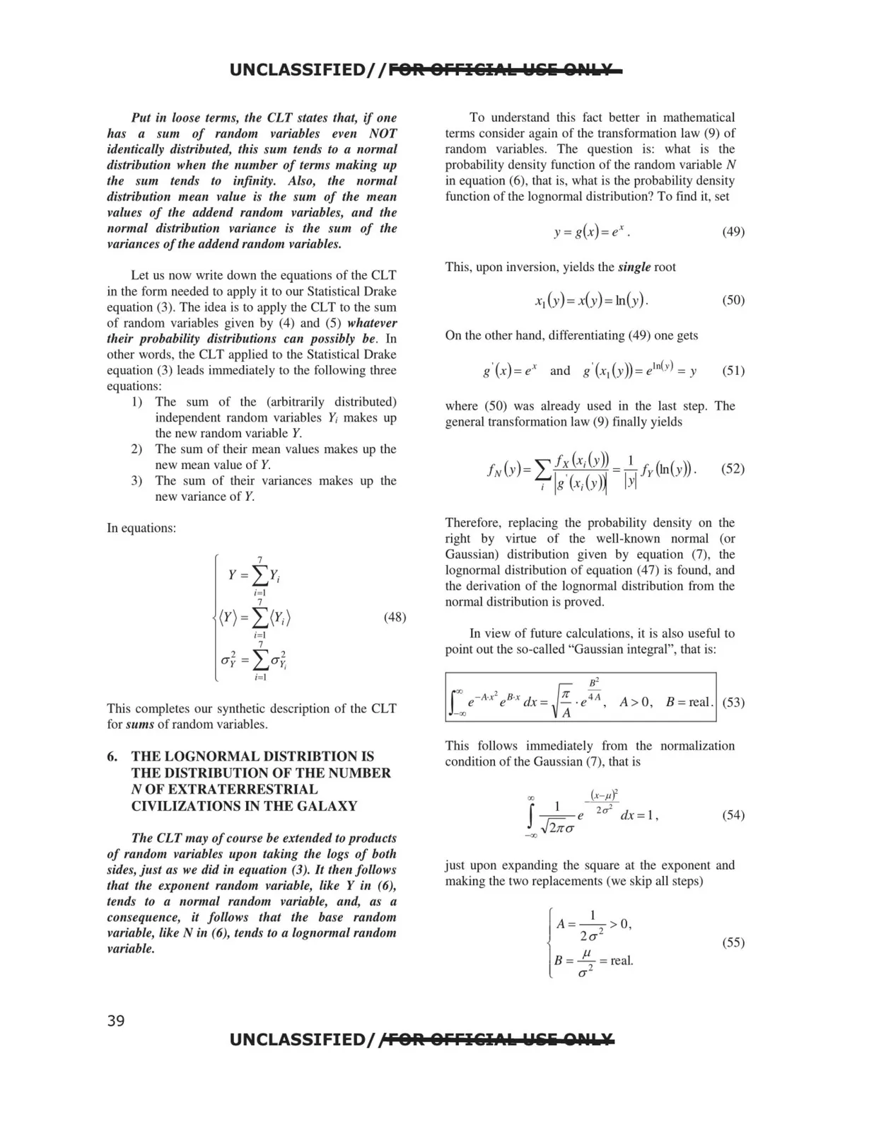
UNCLASSIFIED/ /fOR OFFI&IAk Wlii QPU,¥
Put in loose terms, the CLT states that, if one
has a sum of random variables eve11
NOT
identically distributed, this sum tends to a normal
distribution whe11 the 11umber of tenns maki11g up
the sum te11ds to infinity. Also, the normal
distribution mean value is the sum of the mean
values of the addend random variables, and the
normal distribution variance is the sum of the
variances ofthe addend random variables.
Let us now write down the equations of the CLT
in the form needed to apply it to our Statistical Drake
equation (3). The idea is to apply the CLT to the sum
of random variables given by (4) and (5) whatever
their probability distributions ca11 possibly be. Tn
other words, the CL T applied to the Statistical Drake
equation (3) leads immediately to the following three
equations:
I) The sum of the (arbitrarily distributed)
independent random variables Y; makes up
the new random variable Y.
2) The sum of their mean values makes up the
new mean value of Y.
3) The sum of their variances makes up the
new variance of Y.
In equations:
7
y = :~::vi
i =I
7
(Y) = I(Y; )
(48)
i=I
7
2 ="'
O'y
L..Jo-r2,
i= I
This completes our synthetic description of the CL T
for sw11s of random variables.
6. THE LOGNORMAL DISTRIBTIO IS
THE DISTRIBUTION OF THE NUMBER
N OF EXTRATERRESTRIAL
CIVILIZATIONS IN THE GALAXY
The CLT may ofcourse be exte11ded to products
of random variables upon taki11g the logs of both
sides, just as we did in equatio11 (3). It then follows
that the exponent random variable, like Y i11 (6),
tends to a 11ormal random variable, and, as a
co11seque11ce, it follows that the base random
variable, like N i11 (6), te11ds to a lognormal random
variable.
To understand this fact better in mathematical
terms consider again of the transformation law (9) of
random variables. The question is: what is the
probability density function of the random variable N
in equation (6), that is, what is the probability density
function of the lognormal distribution? To find it, set
(49)
This, upon inversion, yields the single root
x1(y) =x(y) =!n(y).
(50)
On the other hand, differentiating (49) one gets
where (50) was already used in the last step. The
general transformation law (9) finally yields
( ) "' fx(x;(y))
1
( ( ))
fNY= L..J i '( ()~=- /ylny •
(52)
i
g X; )' ~
11y
Therefore, replacing the probability density on the
right by virtue of the well-known normal (or
Gaussian) distribution given by equation (7), the
lognormal distribution of equation (47) is found , and
the derivation of the lognormal distribution from the
normal distribution is proved.
In view of future calculations, it is also useful to
point out the so-called "Gaussian integral", that is:
B2
f"' e - Ax2 e 8 ·x dx = ~ •e 4 A
A> 0
B =real. (53)
L.,
VA
'
'
This follows immediately from the normalization
condition of the Gaussian (7), that is
oo
(x-pf
1
--
,­
J-- e lu· dx=l
(54)
&a-
'
--Oj
just upon expanding the square at the exponent and
making the two replacements (we skip all steps)
l
A= -- >0,
2
2a­
(55)
l
B = ; 2 = real.
UNCLASSIFIED/ /FOR 8FFIGl.t.k W&i ,n11.¥
39