AAWSAP DIRD, An Introduction to the Statistical Drake Equation, March 2010

Text

This text came with the file. It may have mistakes. When the text and the image disagree, the image is right.

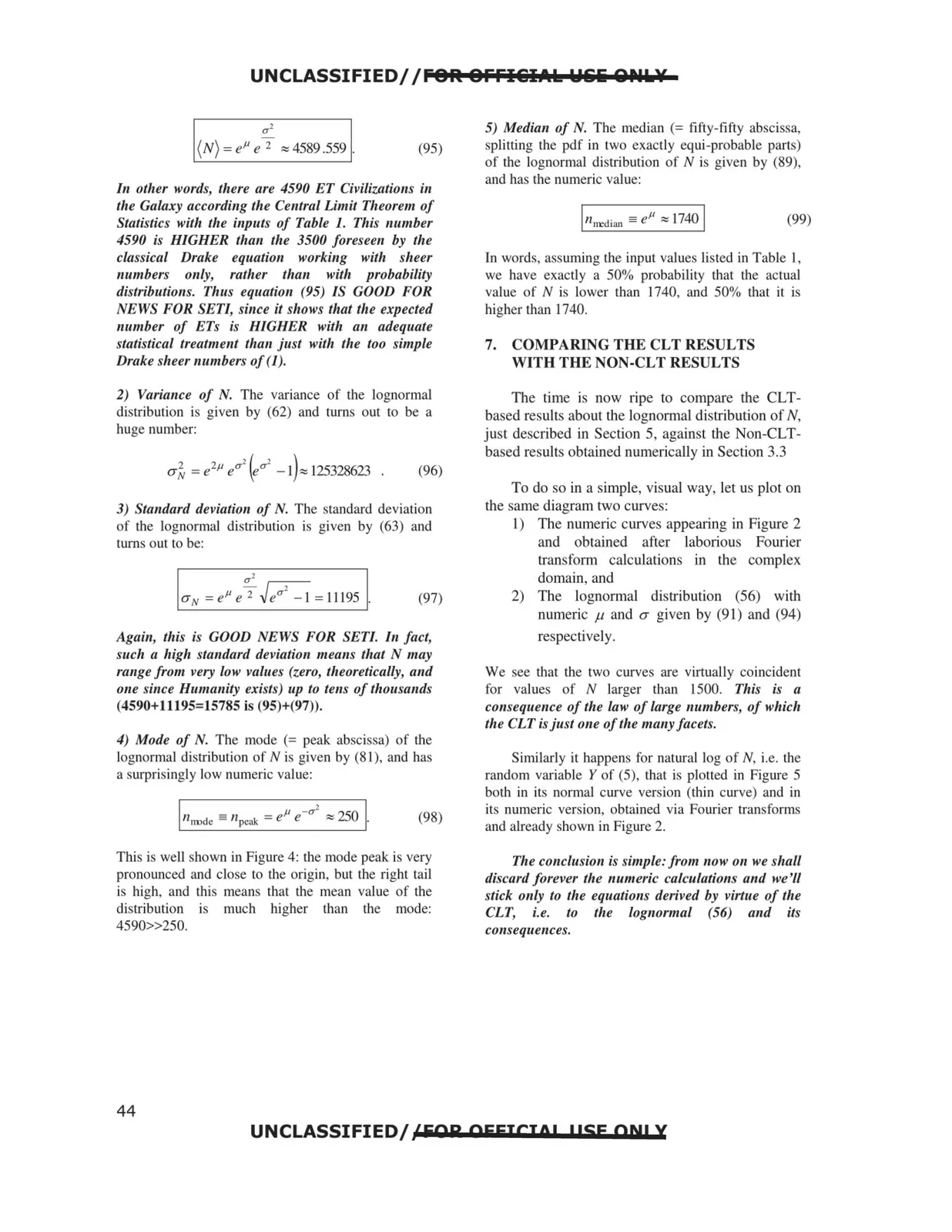
UNCLASSIFIED/ /FOR OFFIEiIAk Wlii QPU,¥
(N) =eµ e 2 "'4589 .559 .
(95)
In other words, there are 4590 ET Civilizatio11s in
the Galaxy according the Central Limit Theorem of
Statistics with the inputs of Table 1. This ,mmber
4590 is HIGHER than the 3500 foreseen by the
classical Drake equation working with sheer
numbers only,
rather than
with
probability
distributions. Thus equation (95) IS GOOD FOR
NEWS FOR SETI, since it shows that the expected
number of ETs is HIGHER with an adequate
statistical treatment than just with the too simple
Drake sheer numbers of(1).
2) Variance of N. The variance of the Iognormal
distribution is given by (62) and turns out to be a
huge number:
3) Standard deviation of N. The standard deviation
of the lognormal distribution is given by (63) and
turns out to be:
(97)
Again, this is GOOD NEWS FOR SETI. In fact,
such a high standard deviation means that N may
range from very low values (zero, theoretically, and
one since Humanity exists) up to tens of thousands
(4590+11195=15785 is (95)+(97)).
4) Mode of N. The mode (= peak abscissa) of the
lognormal distribution of N is given by (81 ), and has
a surprisingly low numeric value:
This is well shown in Figure 4: the mode peak is very
pronounced and close to the origin, but the right tail
is high, and this means that the mean value of the
distribution
is
much
higher
than
the
mode:
4590»250.
5) Median of N. The median (= fifty -fifty abscissa,
splitting the pdf in two exactly equi-probable parts)
of the lognormal distribution of N is given by (89),
and has the numeric value:
(99)
Tn words, assuming the input values listed in Table 1,
we have exactly a 50% probability that the actual
value of N is lower than 1740, and 50% that it is
higher than 1740.
7. COMPARING THE CLT RESULTS
WITH THE NON-CLT RESULTS
The time is now ripe to compare the CLT­
based results about the lognormal distribution of N,
just described in Section 5, against the Non-CLT­
based results obtained numerically in Section 3.3
To do so in a simple, visual way, let us plot on
the same diagram two curves:
1) The numeric curves appearing in Figure 2
and obtained after laborious Fourier
transform calculations in the complex
domain, and
2) The lognormal distribution (56) with
numeric µ and a given by (91) and (94)
respectively.
We see that the two curves are virtually coincident
for values of N larger than 1500. This is a
consequence of the law of large numbers, of which
the CLT is just one ofthe 111a11y facets.
Similarly it happens for natural log of N, i.e. the
random variable Y of (5), that is plotted in Figure 5
both in its normal curve version (thin curve) and in
its numeric version, obtained via Fourier transforms
and already shown in Figure 2.
The conclusion is simple: from now 011 we shall
discard forever the 1111meric calc11lations a11d we'll
stick only to the equations derived by virtue of the
CLT,
i.e.
to
the
lognormal
(56)
and
its
co11seque11ces.
UNCLASSIFIED//509 OFFICIO! 11SF QN1X
44